Bayes factors for the hypotheses of a Bayesian hierarchical SDT model

Tests point, directional and interval hypotheses about the quantities of the three uSDT hypotheses in a Bayesian hsdt() fit or a custom model fitted with brms: the difference between mean sensitivities (diff, H1, reported as $\Delta d'$, influence minus awareness), their correlation (rho, H2) and the slope and intercept of the latent regression (slope, intercept, H3).

Usage

usdt_bf(
  fit,
  hypothesis = c("diff = 0", "rho = 0", "intercept = 0"),
  awareness = "d_A",
  influence = "d_I",
  level = NULL,
  plot = TRUE
)

# S3 method for class 'usdt_bf'
print(x, digits = 3L, width = 80L, ...)

Arguments

fit: A Bayesian hsdt object, fitted with estimation = "bayesian", or a brmsfit whose priors meet the conditions in Details.
hypothesis: Character vector of hypotheses. Each one is "<quantity> <op> <value>", where the quantity is diff, rho, slope or intercept and the operator is =, < or > (<= and >= are read as < and >), or "<quantity> in [a, b]" and "<quantity> out [a, b]" for a region and its complement. A point statement is the null hypothesis H0, and H1 its negation. An inequality or a region is the alternative H1, and H0 its complement. The default tests the three point nulls.
awareness, influence: For a brms model, the population-level terms of the awareness and influence sensitivities, as in usdt_tests(). Ignored for an hsdt fit.
level: Credible level of the reported intervals. Defaults to the level of an hsdt fit, and to 0.95 for a brms model.
plot: Logical. Draw, for each hypothesis, a panel with the prior and posterior of the tested quantity (default TRUE). Set plot = FALSE inside loops, reports and other functions, and draw the figure later with plot.usdt_bf().
x: A usdt_bf object.
digits: Number of decimals printed.
width: Width of the printed report, in characters.
...: Ignored.

Value

An object of class usdt_bf: a data frame with one row per hypothesis and the columns hypothesis, test ("Savage-Dickey density ratio test", "Directional test" or "Interval test"), H1, H0, estimate and est.error (posterior mean and SD), conf.low and conf.high (central credible interval), post.prob (posterior probability of H1 for a directional or interval test), log_BF10, BF10, BF01, evidence and favours. It prints one report per hypothesis, with both log Bayes factors. The prior and posterior curves are stored, so plot.usdt_bf() can draw the figure again.

Point hypotheses: the Savage-Dickey density ratio

A point hypothesis $\theta = c$ compares a model in which $\theta$ is fixed at $c$ with the fitted model, in which it is free. When the first is nested in the second and keeps the conditional prior of the other parameters, the Bayes factor is the ratio of the posterior and prior densities at $c$ (Dickey & Lientz, 1970, Wagenmakers et al., 2010): $$\mathrm{BF}_{01} = p(\theta = c \mid y) / p(\theta = c).$$ The posterior density comes from a logspline fit to the posterior draws. A fit is used only if its distribution function stays within 0.05 of that of the draws at every percentile. When neither logspline algorithm gives such a fit, which happens with the very heavy tails of the intercept and slope when the awareness sensitivities barely vary across subjects, the draws are fitted on the scale $\mathrm{asinh}((x - m)/s)$, with $m$ their median and $s$ their median absolute deviation, and the density is mapped back. Density estimates are least precise far from the posterior mass, so a test value deep in a tail is read on the log scale and with caution.

Directional and interval hypotheses

An inequality or a region is evidence about where the quantity lies, so its Bayes factor is the ratio of posterior to prior odds of H1: $$\mathrm{BF}_{10} = \frac{P(H_1 \mid y) / P(H_0 \mid y)}{P(H_1) / P(H_0)}.$$ post.prob reports $P(H_1 \mid y)$, the share of posterior draws in H1, and the prior probabilities come from the priors described below. When every draw falls on one side, the draws cannot bound the Bayes factor and log_BF10 is infinite.

The prior of each quantity

rho: the marginal of the lkj prior of usdt_priors(), exact.
diff: given the mean awareness sensitivity $\mu_A$, the difference is the mean influence sensitivity shifted by $\mu_A$, so its prior density and probabilities are those of the prior of $\mu_I$ at $x + \mu_A$, averaged over 100,000 prior draws of $\mu_A$ (a Rao-Blackwell estimate). With normal priors on both means this is the normal prior of their difference.
intercept: induced by the other priors. Given the slope $\beta_1$ and $\mu_A$, the intercept is $\mu_I$ shifted by $\beta_1 \mu_A$, so its prior is likewise averaged over 100,000 prior draws of the slope and of $\mu_A$. The prior has no mean or variance, because the slope involves $1/\sigma_A$.
slope: given the ratio $\sigma_I / \sigma_A$, the slope is a rescaled correlation, so its prior is averaged over 100,000 prior draws of that ratio. Its density is infinite at zero, and the slope always has the sign of the correlation, so slope = 0, slope > 0 and slope < 0 are tested as the same statements about rho. The row still summarises the posterior of the slope.

Under the latent regression parameterization the intercept has a prior of its own instead of $\mu_I$, so it is exact like rho, and slope is as above. The difference is induced:

diff: $\beta_0 + (\beta_1 - 1) \mu_A$, so its prior is that of the intercept, shifted and averaged over 100,000 prior draws of the slope and of $\mu_A$. Like the induced intercept above, it has heavy tails and no mean or variance.

The data fix $\mu_I = \beta_0 + \beta_1 \mu_A$, so under the latent regression a narrow intercept prior also moves the posterior of the slope and of rho, even though their priors are independent of it: the Bayes factors of rho and slope then depend on the intercept prior as well.

These averages work for any family of usdt_priors(). The prior draws use the random number generator. Call set.seed() first for reproducible results.

Custom brms models

For a brmsfit, the priors are read from brms::prior_summary(), each parameter taking its most specific prior (coefficient, then group, then class), and the quantities get the same priors as above. The model must have:

a proper prior on each sensitivity term, from the families of usdt_priors(), e.g. prior(normal(0, 1), class = b). The flat default of brms is improper, and a Bayes factor needs a proper prior.
an LKJ($\eta$) prior on the correlations of the group-level term that holds both sensitivities. One correlation of a $K \times K$ LKJ matrix has the marginal of a $2 \times 2$ LKJ($\eta - 1 + K/2$), so a block with other terms besides the two sensitivities still has an exact prior for rho.
for intercept and slope, priors on the two SDs from the families of usdt_priors(), truncated at zero as brms does. The brms default, student_t(3, 0, 2.5), qualifies.

The Bayes factor of a point hypothesis depends on the prior of the tested quantity: a wider prior puts less density at the tested value and favours the null. The intercept prior is induced by the means, SDs and correlation, so its Bayes factor depends on all of them. Report results with the priors used, and check them with other reasonable priors.

evidence follows the bands of Jeffreys (1961) with the labels of Lee and Wagenmakers (2013): anecdotal ($\mathrm{BF} < 3$), moderate (< 10), strong (< 30), very strong (< 100) and extreme.

References

Dickey, J. M., & Lientz, B. P. (1970). The weighted likelihood ratio, sharp hypotheses about chances, the order of a Markov chain. The Annals of Mathematical Statistics, 41(1), 214-226. doi:10.1214/aoms/1177697203

Jeffreys, H. (1961). Theory of probability (3rd ed.). Oxford University Press.

Lee, M. D., & Wagenmakers, E.-J. (2013). Bayesian cognitive modeling: A practical course. Cambridge University Press.

Wagenmakers, E.-J., Lodewyckx, T., Kuriyal, H., & Grasman, R. (2010). Bayesian hypothesis testing for psychologists: A tutorial on the Savage-Dickey method. Cognitive Psychology, 60(3), 158-189. doi:10.1016/j.cogpsych.2009.12.001

Examples

# \donttest{
d <- usdt_data_tasks(
  awareness = vadillo_awareness,
  influence = vadillo_cuing,
  subject_col      = "subj",
  condition_col    = "condition",
  condition_levels = c(signal = "old", noise = "new"),
  response_col     = list(awareness = "judged.old", influence = "rt"),
  response_levels  = list(awareness = c(signal = 1, noise = 0),
                          influence = c(signal = "faster",
                                        noise = "slower")),
  dichotomize      = list(awareness = FALSE, influence = TRUE)
)

m <- hsdt(d, estimation = "bayesian", seed = 1)
#> ── Fitting the Bayesian hierarchical SDT model ──────────────────────── rstan ──
#> ℹ 4 chains of 5000 draws after 1000 warmup iterations, 2 at a time.
#> ✔ Sampled 4 chains in 55.1s.
#> ✔ No divergent transitions.
#> ✔ No transition reached the maximum tree depth (10).
#> ✔ Largest R-hat 1.002, below 1.01.
#> ✔ Smallest effective sample size 1605, above 400.

# The three point nulls, with their figure
set.seed(1)
usdt_bf(m)

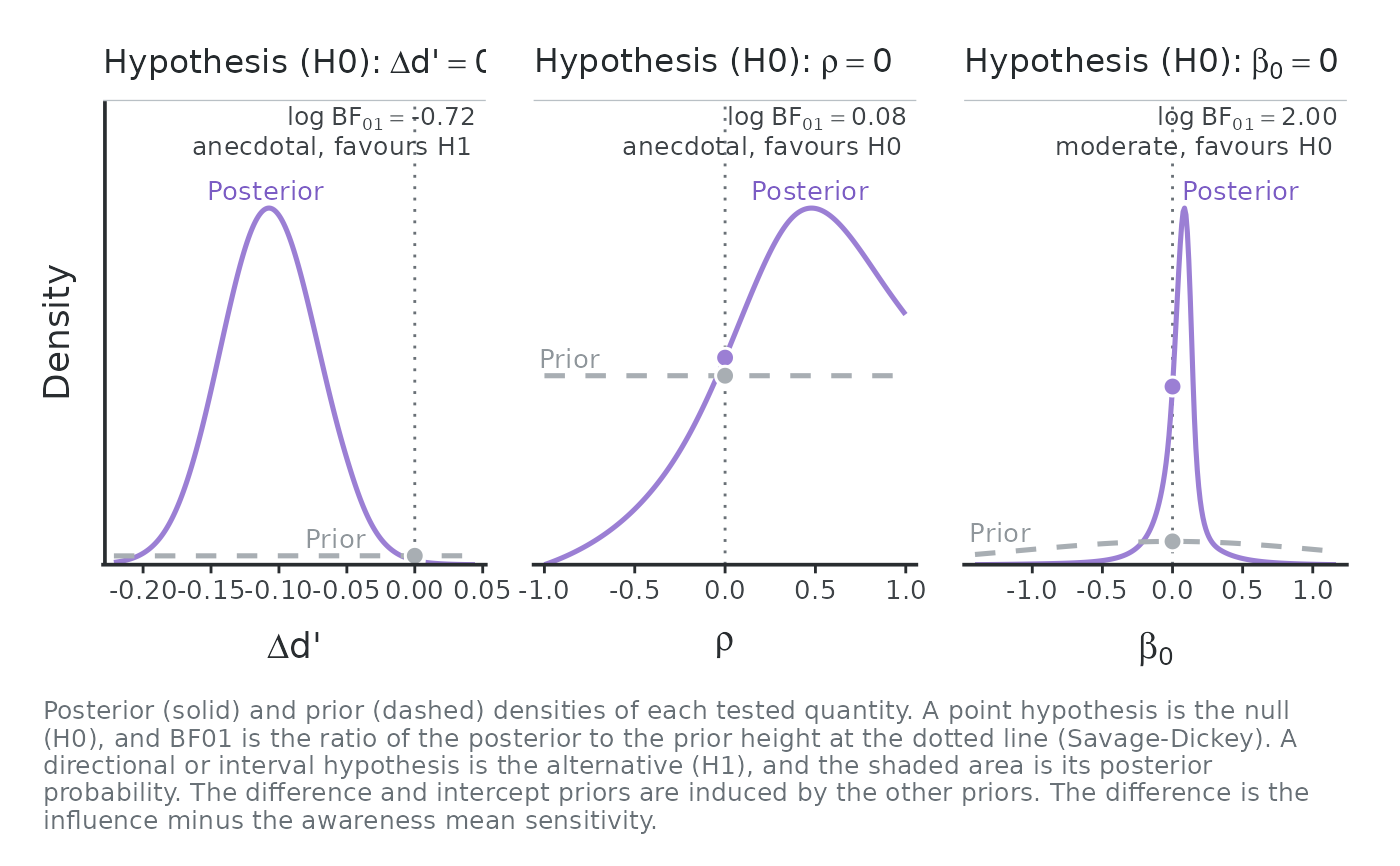#>  uSDT hypothesis ─ Savage-Dickey density ratio test
#> ════════════════════════════════════════════════════════════════════════════════
#>   Hypothesis (H1)             : Δd' != 0
#>   Hypothesis (H0)             : Δd' = 0
#>   Posterior mean              : -0.107
#>   Posterior SD                : 0.036
#>   95% CrI                     : [-0.177, -0.036]
#>   log BF10                    : 0.724
#>   log BF01                    : -0.724
#>   Evidence                    : anecdotal for H1
#> ────────────────────────────────────────────────────────────────────────────────
#> 
#>  uSDT hypothesis ─ Savage-Dickey density ratio test
#> ════════════════════════════════════════════════════════════════════════════════
#>   Hypothesis (H1)             : rho != 0
#>   Hypothesis (H0)             : rho = 0
#>   Posterior mean              : 0.309
#>   Posterior SD                : 0.447
#>   95% CrI                     : [-0.726, 0.964]
#>   log BF10                    : -0.079
#>   log BF01                    : 0.079
#>   Evidence                    : anecdotal for H0
#> ────────────────────────────────────────────────────────────────────────────────
#> 
#>  uSDT hypothesis ─ Savage-Dickey density ratio test
#> ════════════════════════════════════════════════════════════════════════════════
#>   Hypothesis (H1)             : intercept != 0
#>   Hypothesis (H0)             : intercept = 0
#>   Posterior mean              : -0.035
#>   Posterior SD                : 3.693
#>   95% CrI                     : [-0.980, 0.737]
#>   log BF10                    : -1.996
#>   log BF01                    : 1.996
#>   Evidence                    : moderate for H0
#> ────────────────────────────────────────────────────────────────────────────────

# Unconscious processing as a directional hypothesis, and a region of
# practical equivalence for the difference, without the figure
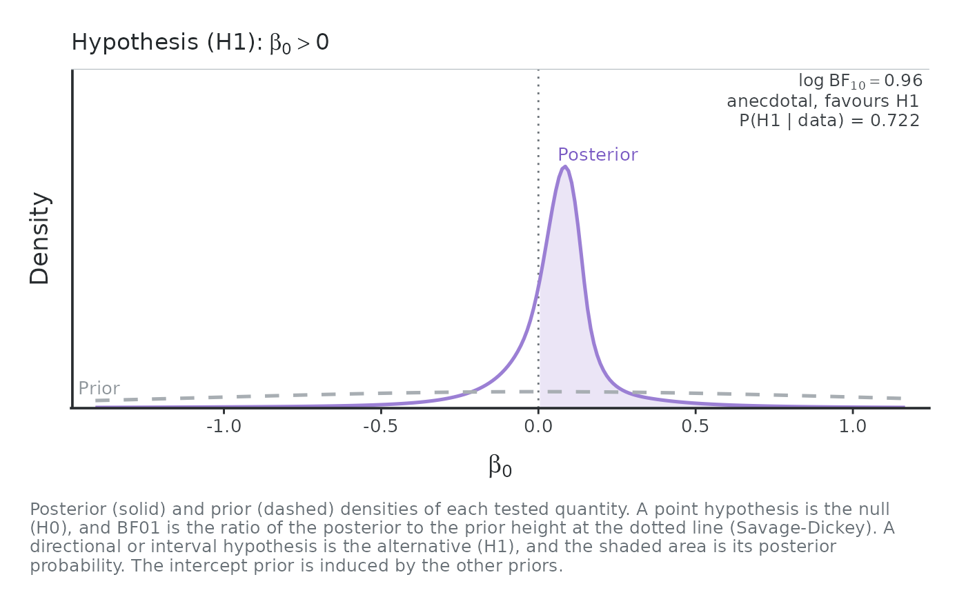
b <- usdt_bf(m, c("intercept > 0", "diff in [-0.1, 0.1]"), plot = FALSE)
b
#>  uSDT hypothesis ─ Directional test
#> ════════════════════════════════════════════════════════════════════════════════
#>   Hypothesis (H1)             : intercept > 0
#>   Hypothesis (H0)             : intercept <= 0
#>   Posterior mean              : -0.035
#>   Posterior SD                : 3.693
#>   95% CrI                     : [-0.980, 0.737]
#>   Posterior probability (H1)  : 0.722
#>   log BF10                    : 0.955
#>   log BF01                    : -0.955
#>   Evidence                    : anecdotal for H1
#> ────────────────────────────────────────────────────────────────────────────────
#> 
#>  uSDT hypothesis ─ Interval test
#> ════════════════════════════════════════════════════════════════════════════════
#>   Hypothesis (H1)             : Δd' in [-0.1, 0.1]
#>   Hypothesis (H0)             : Δd' out [-0.1, 0.1]
#>   Posterior mean              : -0.107
#>   Posterior SD                : 0.036
#>   95% CrI                     : [-0.177, -0.036]
#>   Posterior probability (H1)  : 0.426
#>   log BF10                    : 2.520
#>   log BF01                    : -2.520
#>   Evidence                    : strong for H1
#> ────────────────────────────────────────────────────────────────────────────────
plot(b[1, ])

# }