Prior predictive check for the Bayesian hierarchical SDT model

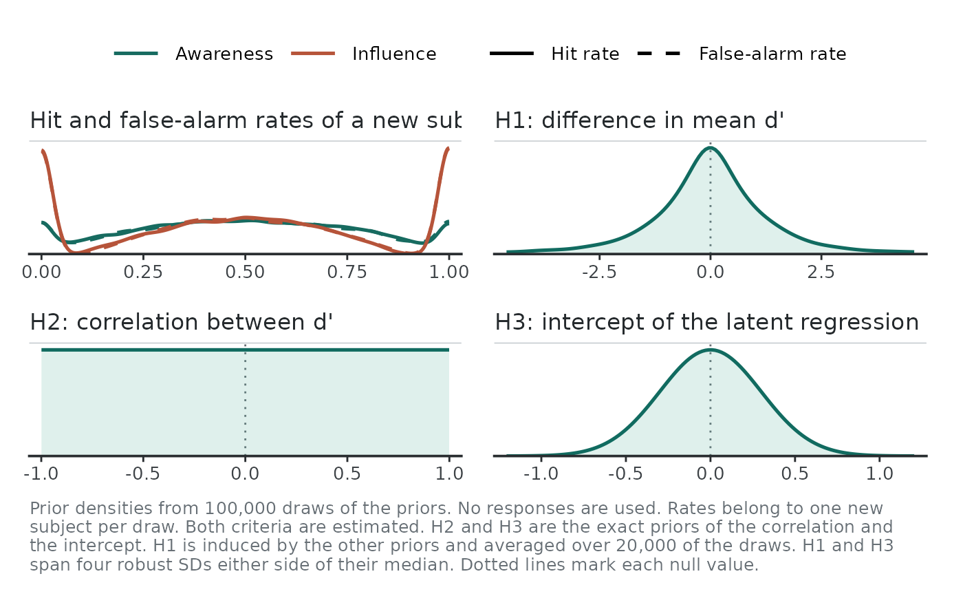
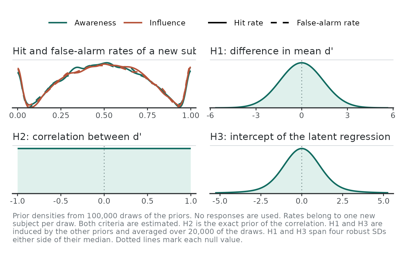
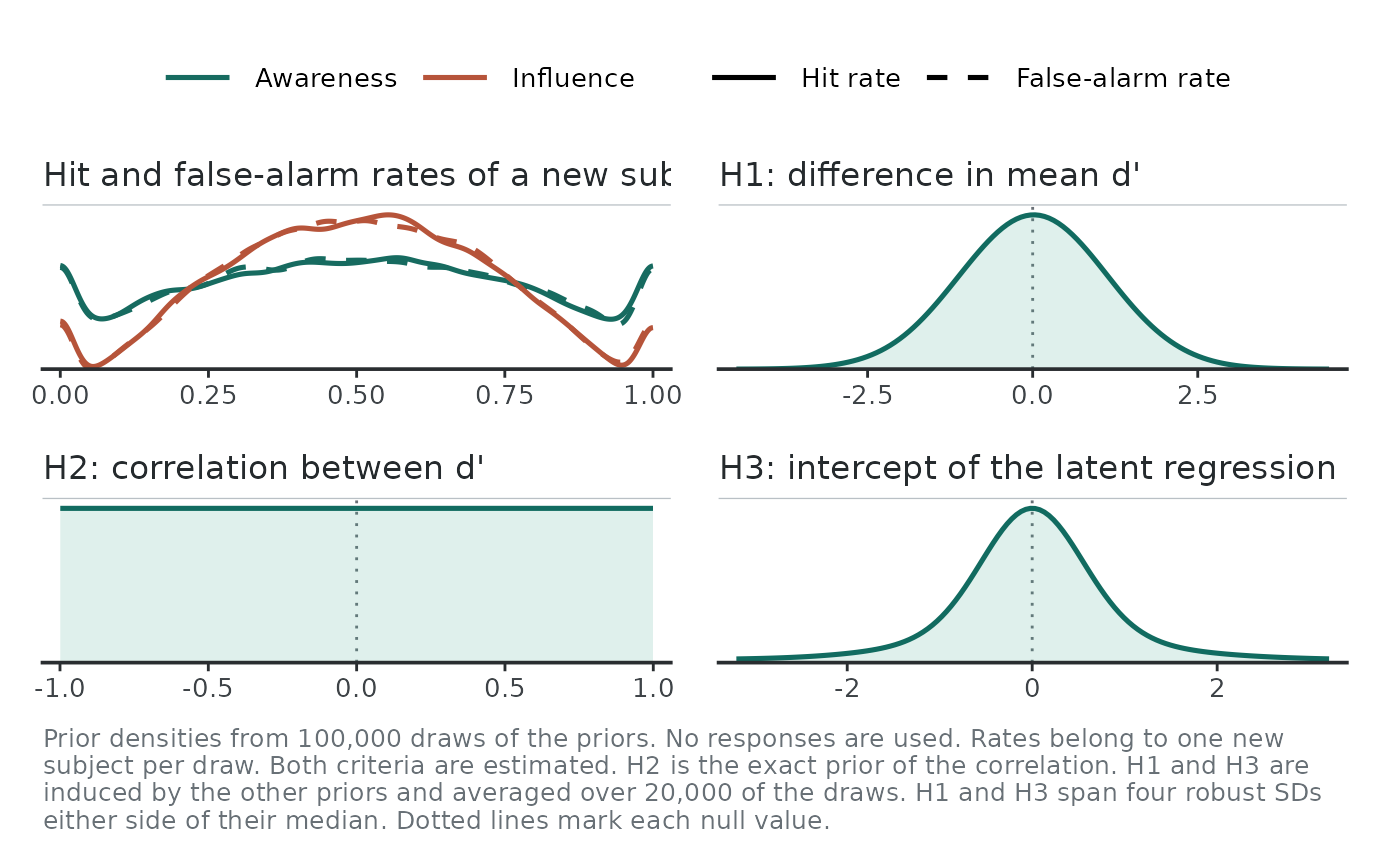
Draws what the priors imply before seeing any data: the hit and false-alarm rates of a new subject in each task, and the prior of the quantity tested by each hypothesis. Use it to check that the priors allow the data you expect and to see the prior that the model induces on the latent intercept.

Usage

# S3 method for class 'usdt_priors'
plot(
  x,
  data = NULL,
  unequal_variances = FALSE,
  latent = c("correlation", "regression"),
  caption = TRUE,
  ...
)

Arguments

x: A usdt_priors object from usdt_priors().
data: Optional usdt_data object. When given, a criterion fixed by the median split stays fixed, as in hsdt(), and the tasks take the data labels. Without it, both criteria are estimated. The caption says which criteria are fixed.
unequal_variances: Logical. Simulate the signal standard deviation from its prior instead of fixing it to 1.
latent: How the model writes the relation between the two latent sensitivities, as in hsdt(): by their means, standard deviations and correlation ("correlation", the default) or by the latent regression of the influence on the awareness one ("regression").
caption: Logical. Show the caption that explains the plot under it (default TRUE).
...: Ignored.

Value

A ggplot object. Its underlying data frame is stored in $data.

Details

The plot simulates 100,000 draws from the priors in R. No model is fitted and Stan is not needed.

The rates panel shows the hit and false-alarm rates of one new subject drawn from each population draw. Rates piled up at 0 or 1 mean that the priors allow extreme performance.

Each hypothesis panel shows the prior of the quantity it tests. A quantity with a prior of its own is drawn exactly: the correlation (H2), and under the latent regression also the intercept (H3). The others have priors that the model induces through the remaining priors: the intercept under the correlation parameterization, the difference (H1) under the latent regression. Each of these is drawn as the density that one prior gives it, averaged over 20,000 prior draws of the other parameters (a Rao-Blackwell estimate), the same priors that usdt_bf() averages over 100,000 draws. The difference (H1) and the intercept (H3) span four robust standard deviations either side of their median, since an induced prior of either has heavy tails. Dotted lines mark the value of each hypothesis under the null.

Examples

plot(usdt_priors())


# A narrower prior for the mean influence sensitivity
plot(usdt_priors(dprime = list(awareness = "normal(0, 1)",
                               influence = "normal(0, 0.5)")))


# The latent regression, with a prior on its intercept
plot(usdt_priors(intercept = "normal(0, 0.3)"), latent = "regression")